
Being in the class of 2021E, I started my mathematics thesis in Spring 2020, and actually concluded it in Fall 2020, officially handing it in on the 11th of November. It was under the supervision of two advisors: Professor Ivan Contreras, a close mentor whose work with a prior summer I hoped to continue in my thesis, and Professor Alejandro Morales of UMass Amherst, a close friend of Professor Contreras and another mentor I grew close to after taking one of his graduate courses on the symmetric group at UMass a few semesters prior.
My thesis was titled Discrete Morse Theory: Enumeration of Discrete Gradient Vector Fields. There tend to be two types of thesis in mathematics: expository (i.e. reading on an advanced topic then writing a more accessible summary) or research (specifically studying the foundations of a topic then pursuing an open question). Both are fantastic and fun approaches (and both may lead to publishable material) — my thesis largely fell into the latter but had a fair amount of exposition as well. I will mainly focus on the research aspects, but my entire thesis is publicly available here for those who want to see it all.
Though I focused primarily on staying within the realm of “pure” mathematics (i.e. doing mathematics for the sake of mathematics) — the work we did has very strong connections to applications. Discrete Morse theory in particular is currently a “hot” topic in the applied sectors of mathematics. It assists in understanding the “shape” of statistical data in fields such as topological data analysis. At a recent conference where I presented my thesis work, I learned from Jim Gates in the audience (!) that the results relate strongly to his work on adinkras, a mathematical object used in studying supersymmetry in physics. Furthermore, discrete Morse theory has been coming up in the study of configuration spaces of hard spheres — which assists in researching possible states for robotic arms and is of interest in engineering applications and physics.
The research problem we were concerned with involved trying to count these notions of discrete gradient fields, which live on structures called simplicial complexes. Tackling this involved not just consulting books — but a close survey of academic papers, scheduling and meetings with experts on these subjects at national conferences, and months of coding in mathematical programming languages like SageMath and Macaulay2. Let’s just focus on the core ideas behind the mathematics here though.
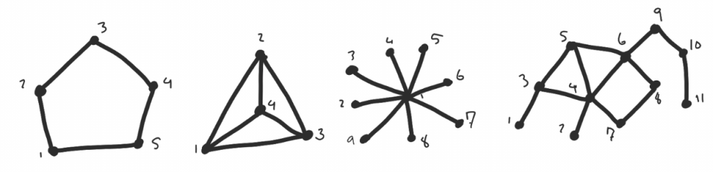
First, let’s try to understand the playing field in which we’ll encounter these discrete gradients: simplicial complexes. A natural place to begin is with the concept of a graph, which is defined to be a collection of points (called vertices) and lines connecting those points (called edges). In the below figure, for instance, we have from left to right: the cycle graph on five vertices, the complete graph on four vertices, the star graph on nine vertices, and some arbitrary graph I made up.
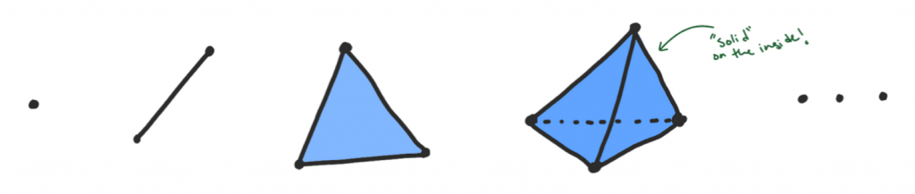
Simplicial complexes can be seen as a generalization of the notion of a graph — where rather than just have 0-dimensional simplices (vertices in our graphs), and 1-dimensional simplices (the edges in our graphs), we go further and allow our structure to have higher dimensional simplices as well. Notice that the “boundary” of a 1-dimensional simplex (edge) are two 0-dimensional simplices (vertices). This idea is carried on forward: the 2-dimensional simplex looks like a solid triangle, and its boundary consists of three 1-dimensional simplices. The 3-dimensional simplex looks like a solid tetrahedron, and its boundary consists of four 2-dimensional simplices. In general, if you have some positive integer n, that defines an n-dimensional simplex! In the below figure, we have from left to right: a 0-dimensional simplex, 1-dimensional simplex, 2-dimensional simplex, and a 3-dimensional simplex.
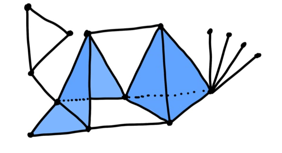
Having all these new parts opens up a world of crazy-look possibilities, of course, the vast majority of them live in too high of dimensions for us to straightforwardly draw. Though just for intuition’s sake, here is an arbitrary example of what a simplicial complex could look like:
My main focus was trying to understand the discrete gradient vector fields that live on such a simplicial complex. One can draw an analogy from calculus: just as a nice function in the plane gives rise to a gradient vector field, having a discrete Morse function on a simplicial complex gives rise to a discrete gradient vector field.
A discrete Morse function on a simplicial complex (though it may help to restrict to graphs to first get a grasp) is an assignment of real numbers to all the simplicies, such that two conditions are met at every simplex A:
- At most one higher dimensional neighbor has a lower or equal value than the value at A.
- At most one lower-dimensional neighbor has a higher or equal value than the value at A.
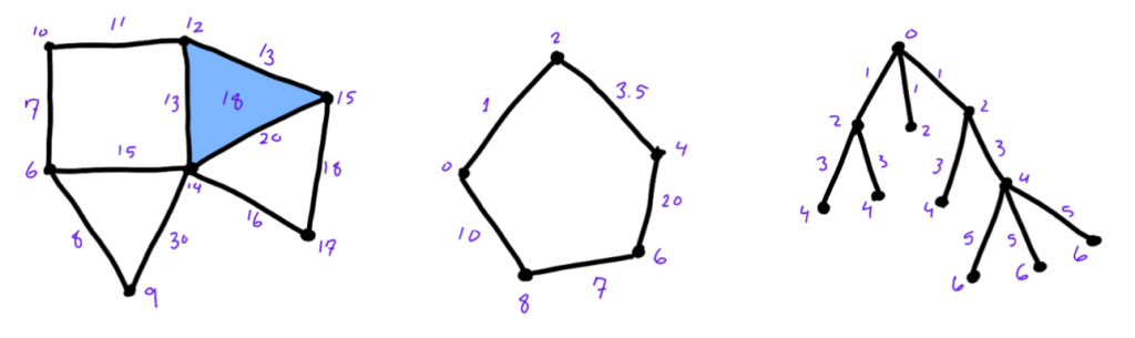
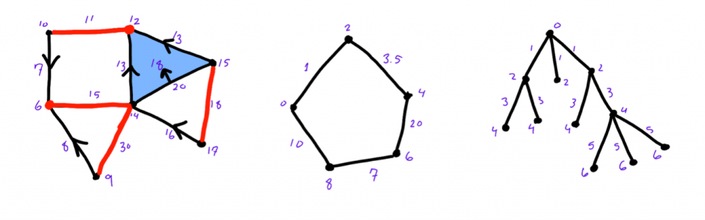
This is a tough definition to immediately get a good understanding of, so don’t get discouraged! I recall spending the better part of my day at the Black Sheep Deli the first summer I grappled with this — and even then it took days of doing more examples before I felt like I “understood” what it was really saying. Let’s look at a few examples of discrete Morse functions. I strongly encourage you to check for at least one of these that the conditions are satisfied everywhere — and perhaps even construct your own graph (or simplicial complex, if you’re ambitious) and some discrete Morse functions on it!
Now finally, we can introduce the main contender: given a discrete Morse function on simplicial complexes (which, recall, includes graphs), you obtain the discrete gradient vector field of that discrete Morse function by applying this one rule everywhere:
- If A is an n-dimensional simplex and B is an (n+1)-dimensional simplex neighbor, then we point an arrow from A to B if and only if B is assigned a value smaller than or equal to A.
Some simplices may not end up being the head/tail of an arrow, and those simplices are special. I encourage you to figure out when that happens and why that happens — you certainly have all the information you need here in this article.
I’ve gone ahead and found one of the discrete gradients from the simplicial complexes up above, but I’ve graciously left the others to haunt you until you solve them. I’ve highlighted the aforementioned “special” simplicies to encourage you to think more about them as well — they’re quite critical to the thesis work.
In the end, we were able to succeed in understanding the structure of these discrete gradient vector fields quite deeply, as well as figured out exactly how to count them. This road was long and winding — and required even grappling with famous objects like the Mobius band and Klein bottle to ultimately arrive at our conclusion. I won’t state what we found, but rather encourage you to explore these gradients on your own time. Ask questions, pose conjectures, and try to prove them. As in the end, this is what my thesis really was all about.
You must be logged in to post a comment.